Part 2 showed pixel prediction smearing on bimodal futures. Part 3 showed that joint embedding training in the same setup hits the same wall: the encoder cannot pull direction information out of a single frame, so any predictor under MSE in any space averages between left and right.
Real JEPAs do not pretend the missing information is in the input. They take it as an extra input to the predictor. That is what V-JEPA 2-AC (Meta FAIR, 2025) does for robot control: alongside the visible video frames, the predictor receives the control signal sent to the robot arm. The future stops being ambiguous given the action.
This part ports that pattern back to the bouncing-ball toy and adds a small planner on top. Code in part4_planning/.
Action-conditioned predictor
Encoder is unchanged: a 64x64 frame goes in, a 128-dim embedding comes out. The predictor now takes the embedding plus a scalar action (-1 for left, +1 for right):
class ActionPredictor(nn.Module):
    def __init__(self, embed_dim=128, hidden=256):
        super().__init__()
        self.net = nn.Sequential(
            nn.Linear(embed_dim + 1, hidden),
            nn.GELU(),
            nn.Linear(hidden, embed_dim),
        )

    def forward(self, z, action):
        a = action.unsqueeze(-1) if action.dim() == 1 else action
        return self.net(torch.cat([z, a], dim=-1))
Training is the same VICReg setup from Part 3. The only differences are the predictor’s signature and the data: I extended simulate_episode to record direction at each step, then trained on (frame_t, frame_t+1, action_t) triples.
Final loss after 6000 steps: sim 0.0057, var 0.010, cov 6.4, z_std 1.01. The sim term is roughly 14x lower than the action-free VICReg run from Part 3 (0.082), and that is the whole point. With direction provided, the predictor’s job becomes deterministic. There is no average-of-two-futures penalty bottlenecking the loss.
Planning in embedding space
The predictor is deterministic given an action. Chain it H times and you get a rollout: a sequence of predicted embeddings starting from encoder(x_0) under any action sequence [a_0, ..., a_{H-1}].
For planning, give it a goal image x_g and ask: which action sequence drives the rollout closest to encoder(x_g)?
seqs = enumerate_actions(horizon)             # (2^H, H)
z = encoder(x_0).expand(seqs.size(0), -1).clone()
for t in range(horizon):
    z = predictor(z, seqs[:, t])
dist = ((z - encoder(x_g)) ** 2).sum(dim=-1)  # (2^H,)
best = seqs[dist.argmin()]
Action space is binary, horizon is small (6), so I just enumerate all 2^6 = 64 sequences and pick the one with lowest L2 distance to the goal embedding in latent space. No gradient-based optimisation, no rollout sampling, no MCTS. The whole planner is fifteen lines.
This is the simplest possible expression of the V-JEPA 2-AC pattern: model-predictive control where the world model lives entirely in embedding space and only the start and goal are ever in pixel form.
What it looks like
I generated a 7-frame ground-truth episode (seed 11, ball happens to be moving right), gave the planner the first and last frames, and let it search.
The planner returned [+1, +1, +1, +1, +1, +1] - all “go right”. Rolling out from the initial embedding under that action sequence and decoding each step back to pixels via a frozen autoencoder decoder:
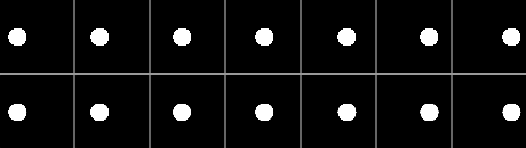
Top row is the ground truth. Bottom row is the model’s rollout decoded back to pixels. They match position by position. Final pixel-space RMS distance from the rolled-out terminal frame to the actual goal frame: 0.0275 - essentially zero on the scale where a fully smeared bimodal frame from Part 2 had RMS around 0.4.
Why this works where Part 2 didn’t
Part 2 asked: predict the next frame from a single frame. The bimodal-direction ambiguity was inside the input; no architecture could pull direction out of pixels that didn’t contain it. MSE-on-pixels averaged. Embedding-space MSE in Part 3 still averaged.
Part 5 asks: predict the next embedding from a frame and the direction. The ambiguity is now resolved by an extra input. The predictor’s job is information-theoretically well-defined, the loss converges low, and the planner can use the predictor as a deterministic forward model.
This is the architectural slot Yann LeCun’s argument has been pointing at the whole time. The world model is learned (the encoder + predictor), the planning is classical (search action sequences), and the prediction step happens entirely in embedding space.
What the toy doesn’t show
A bouncing ball in 1D with a binary action space is the smallest world model imaginable. Real V-JEPA 2-AC takes continuous robot control signals, predicts in the embedding space of a video transformer, and is evaluated on zero-shot pick-and-place. The architecture and the planning loop are the same shape; the encoder, the action space, and the data are bigger.
The toy is small enough to read in one sitting and runs in under five minutes per part on an M3 MacBook. That is the project’s whole point.
What this series did and didn’t show
Five parts:
- The argument and the papers behind it.
- Pixel-MSE smears on bimodal futures, shown mathematically and visually.
- Joint-embedding training, representation collapse, and the Barlow Twins / VICReg / LeJEPA fixes on the same toy.
- A production joint-embedding encoder (DINOv2/v3) discovering semantic structure on a real image without labels.
- Action-conditioned prediction and latent-space planning end-to-end on the bouncing ball.
What the toy could and could not carry came clear along the way. Joint-embedding loss alone does not escape the information-theoretic limits of the input. The win is structural and architectural - the encoder discards unpredictable detail, the predictor accepts conditioning information as a slot, and downstream tasks consume the embedding rather than the decoded pixels. The argument is testable, on a laptop, in under thirty minutes of training across all five parts.
The repo is at danieljohnmorris/tiny-bouncing-jepa with one folder per part of the series.